| ### Solution | | ### Solution |
| | | |
| First, we will solve the problem qualitatively, and then quantitatively. | | First, we will solve the problem qualitatively, and then quantitatively. |
| | | |
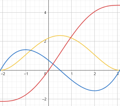
| Let us analyze the velocity graph. By visual inspection, the motion begins at $t=-2.1\ \text{s}$ and ends at $t=3.1\ \text{s}$. The maximum velocity $\upsilon_{\text{max}}=2.4\ \text{m/s}$ is reached at $t=0.5\ \text{s}$. The graph has a symmetric bell-shaped form. | | Let us analyze the velocity graph. By visual inspection, the motion begins at $t=-2.1\ \text{s}$ and ends at $t=3.1\ \text{s}$. The maximum velocity $\upsilon_{\text{max}}=2.4\ \text{m/s}$ is reached at $t=0.5\ \text{s}$. The graph has a symmetric bell-shaped form. |
| | | |
| Acceleration is the derivative of velocity. Geometrically, acceleration is the slope (tangent of the angle) of the tangent line to the velocity graph at a given time. At the beginning, velocity increases and so does the tangent slope, which means acceleration is positive. Around $t=-1\ \text{s}$ the tangent slope reaches its maximum, which corresponds approximately to an angle of $60^{\circ}$; the tangent of this angle (i.e., acceleration) is about $1.73\ \text{m/s}^2$. After that, the rate of change of velocity decreases, so acceleration decreases. When velocity reaches its maximum value, acceleration becomes zero—this occurs at $t=0.5\ \text{s}$. Then velocity starts decreasing, and acceleration becomes negative. Because of the symmetry of the velocity graph, the acceleration graph will also be symmetric. In the negative range, acceleration decreases until it reaches a minimum of about $-1.73\ \text{m/s}^2$ at $t=2\ \text{s}$. After that, acceleration increases again, reaching zero at the end of motion. | | Acceleration is the derivative of velocity. Geometrically, acceleration is the slope (tangent of the angle) of the tangent line to the velocity graph at a given time. At the beginning, velocity increases and so does the tangent slope, which means acceleration is positive. Around $t=-1\ \text{s}$ the tangent slope reaches its maximum, which corresponds approximately to an angle of $60^{\circ}$; the tangent of this angle (i.e., acceleration) is about $1.73\ \text{m/s}^2$. After that, the rate of change of velocity decreases, so acceleration decreases. When velocity reaches its maximum value, acceleration becomes zero—this occurs at $t=0.5\ \text{s}$. Then velocity starts decreasing, and acceleration becomes negative. Because of the symmetry of the velocity graph, the acceleration graph will also be symmetric. In the negative range, acceleration decreases until it reaches a minimum of about $-1.73\ \text{m/s}^2$ at $t=2\ \text{s}$. After that, acceleration increases again, reaching zero at the end of motion. |
| | | |
| Thus, the acceleration graph will be “wave-like” and change sign at the point where velocity reaches its maximum. | | Thus, the acceleration graph will be “wave-like” and change sign at the point where velocity reaches its maximum. |
| | | |
| Position is the integral of velocity. Geometrically, position corresponds to the area under the velocity curve. Since velocity is positive throughout the interval, position always increases and, according to the condition, passes through the point $x(0)=0$. At first, the growth is slow (low velocity), then faster (velocity peak), and then slows again. | | Position is the integral of velocity. Geometrically, position corresponds to the area under the velocity curve. Since velocity is positive throughout the interval, position always increases and, according to the condition, passes through the point $x(0)=0$. At first, the growth is slow (low velocity), then faster (velocity peak), and then slows again. |
| | | |
| Thus, the position graph will be a monotonically increasing S-shaped curve: concave downward at first, then an inflection at maximum velocity, then concave upward. | | Thus, the position graph will be a monotonically increasing S-shaped curve: concave downward at first, then an inflection at maximum velocity, then concave upward. |
| | | |
| Now let us solve quantitatively. | | Now let us solve quantitatively. |
| | | |
| In general, the velocity graph can be approximated by the following function: | | In general, the velocity graph can be approximated by the following function: |
| | | |
| $$\upsilon=\upsilon_{\text{max}}\left[ 1-\left( \frac{t-t_{\text{max}}}{d} \right)^{2} \right]^{2}$$ | | $$\upsilon=\upsilon_{\text{max}}\left[ 1-\left( \frac{t-t_{\text{max}}}{d} \right)^{2} \right]^{2}$$ |
| | | |
| where | | where |
| $\upsilon_{\text{max}}=2.4\ \text{m/s}$ – maximum velocity; | | $\upsilon_{\text{max}}=2.4\ \text{m/s}$ – maximum velocity; |
| $t_{\text{max}}=0.5\ \text{s}$ – the time when maximum velocity is reached; | | $t_{\text{max}}=0.5\ \text{s}$ – the time when maximum velocity is reached; |
| $d=\frac{t_{f}-t_{i}}{2}=\frac{3.1-(-2.1)}{2}=2.6\ \text{s}$ – half-width of the “bell.” | | $d=\frac{t_{f}-t_{i}}{2}=\frac{3.1-(-2.1)}{2}=2.6\ \text{s}$ – half-width of the “bell.” |
| | | |
| Substituting numbers, we get: | | Substituting numbers, we get: |
| | | |
| $$\upsilon(t)=2.4\left[ 1-\left( \frac{t-0.5}{2.6} \right)^{2} \right]^{2}$$ | | $$\upsilon(t)=2.4\left[ 1-\left( \frac{t-0.5}{2.6} \right)^{2} \right]^{2}$$ |
| | | |
| Acceleration: | | Acceleration: |
| | | |
| $$a(t)=\frac{d \upsilon}{dt}=-\frac{2.4}{1.69}(t-0.5)\left[ 1-\left( \frac{t-0.5}{2.6} \right)^{2} \right]$$ | | $$a(t)=\frac{d \upsilon}{dt}=-\frac{2.4}{1.69}(t-0.5)\left[ 1-\left( \frac{t-0.5}{2.6} \right)^{2} \right]$$ |
| | | |
| Position: | | Position: |
| | | |
| $$x(t)=\int \upsilon(t),dt=6.24\cdot \left[ \frac{t-0.5}{2.6}-\frac{2}{3}\left( \frac{t-0.5}{2.6} \right)^{3}+\frac{1}{5}\left( \frac{t-0.5}{2.6} \right)^{5} \right]+C$$ | | $$x(t)=\int \upsilon(t),dt=6.24\cdot \left[ \frac{t-0.5}{2.6}-\frac{2}{3}\left( \frac{t-0.5}{2.6} \right)^{3}+\frac{1}{5}\left( \frac{t-0.5}{2.6} \right)^{5} \right]+C$$ |
| | | |
| The integration constant is found from $x(0)=0$: | | The integration constant is found from $x(0)=0$: |
| | | |
| $$C\approx 1.17$$ | | $$C\approx 1.17$$ |
| | | |
| Finally, the expression for position: | | Finally, the expression for position: |
| | | |
| $$x(t)=6.24\cdot \left[ \frac{t-0.5}{2.6}-\frac{2}{3}\left( \frac{t-0.5}{2.6} \right)^{3}+\frac{1}{5}\left( \frac{t-0.5}{2.6} \right)^{5} \right]+1.17$$ | | $$x(t)=6.24\cdot \left[ \frac{t-0.5}{2.6}-\frac{2}{3}\left( \frac{t-0.5}{2.6} \right)^{3}+\frac{1}{5}\left( \frac{t-0.5}{2.6} \right)^{5} \right]+1.17$$ |
| | | |
| Graphs of acceleration (blue), velocity (yellow), and position (red): | | Graphs of acceleration (blue), velocity (yellow), and position (red): |
| | | |
|  | |  |
| | | |
