Statement
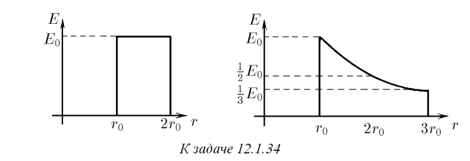
12.1.34. The figure shows the distribution of the electric field of two traveling spherical waves at zero time. Plot the distribution of the electric field at time
Solution
Let us first answer the second question of the problem, since it is simpler.
I will calculate the field energy in CGS units, following the author. It is known that for an electromagnetic wave
If we did not include the magnetic energy, the denominator would be twice as large, but judging by the answer, the author is considering the total energy. On the one hand, this means an inaccuracy in the statement, but generally speaking a purely electric travelling wave without a magnetic component is impossible, so this approach makes sense.
The wave is spherical, so
It should be noted that it is not for nothing that Savchenko marked on the second graph in the problem three points that perfectly lie on the hyperbola
Now we construct the graphs.
First, several important points:
The time
corresponds to a shift of the wave by , where is the speed of propagation of the wave. At the point we see the result of the propagation of the wave from the point . The "extreme" perturbations propagate with the same speed, so the width of the region with nonzero field remains constant.
The total energy of the wave is also constant, so as
increases, the amplitude decreases. The equation of such a wave is
and the second form can be used without assuming that our waves are sinusoidal.
If the distribution at time
Accordingly,
From this expression, the required graphs are very easy to obtain.
First, let us deal with the first wave:
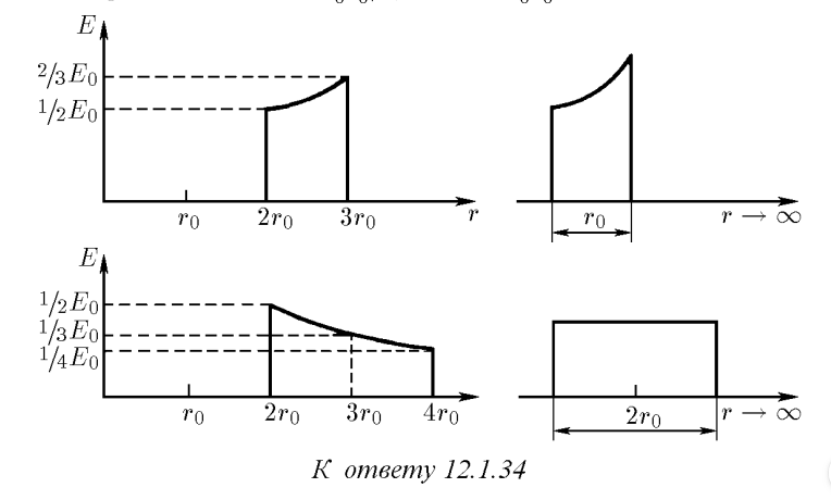
The reference points are easy to calculate by yourself. We have obtained an increasing section instead of a straight line. At infinity, the width of the nonzero region is preserved, and the shape remains approximately the same.
The second wave:
The formula does not change... At infinity, the width of the nonzero region is preserved, and the hyperbola becomes more and more "flat" because the denominator grows. The answer looks like this: