@@ -6,8 +6,7 @@Statement
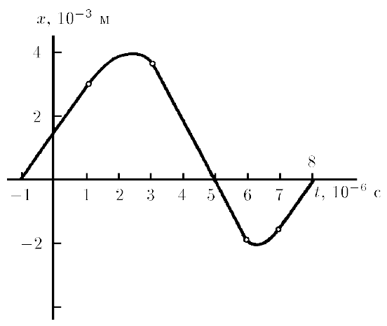
The part of the coordinate-time dependence graph located below the t-axis is similar to the part of the graph that is above this axis (see Figure). Plot graphs based on time, speed, and acceleration. Compare the accelerations for the largest and smallest values of x.
### Solution
−
−
From the plot, it seems reasonable to identify the white open circles with important points and changes on the graph: the graph above the t-axis is linear from $t\in [-1.0,1.0]~\mu\text{s}$, quadratic from $t\in [1.0,3.0]~\mu\text{s}$, and linear from $t\in [3.0,5.0]~\mu\text{s}$. Below the t-axis, the linear slope continues from $t\in [5.0,6.0]~\mu\text{s}$, is quadratic from $t\in [6.0,7.0]~\mu\text{s}$, and finally linear from $t\in [7.0,8.0]~\mu\text{s}$. We ascribe the linear regions with constant velocity, and the quadratic regions with constant acceleration.
+
We'll use $10^{-6}~\text{s} = 1~\mu\text{s}$ and $10^{-3}~\text{m} = 1~\text{mm}$ for values read off of the plot, and will assume 2 significant figures. From the plot, it seems reasonable to identify the white open circles with important points and changes on the graph: the graph above the t-axis is linear from $t\in [-1.0,1.0]~\mu\text{s}$, quadratic from $t\in [1.0,3.0]~\mu\text{s}$, and linear from $t\in [3.0,5.0]~\mu\text{s}$. Below the t-axis, the linear slope continues from $t\in [5.0,6.0]~\mu\text{s}$, is quadratic from $t\in [6.0,7.0]~\mu\text{s}$, and finally linear from $t\in [7.0,8.0]~\mu\text{s}$. We ascribe the linear regions with constant velocity, and the quadratic regions with constant acceleration.
We also note that it looks like the graph maximum is $x= 4.0~\text{mm}$ and the graph minimum is $x= -2.0~\text{mm}$, which is inverted and exactly half as big. Since the problem notes that the regions above and below are similar, we expect all points below the t-axis to be inverted and half as big as the corresponding point above the graph.
The velocities can be easily found in the linear regions by reading off approximate values from the graph, and noting that the plot below the t-axis is negative and half as big.
\begin{align*}
v = \frac{\Delta x}{\Delta t}
\end{align*}
For each linear region we can compute the velocity by reading (approximate) values off of the graph.
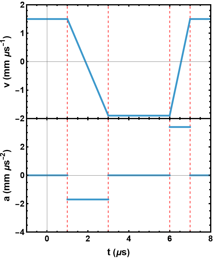
Both of these result are showing in the Figure below. We note that, although the coordinates plotted below the t-axis are half as big, because their times scales are also half as big, the velocities in the ranges $-1.0~\mu\mathrm{s}\leq t \leq 1.0\,\mu\mathrm{s}$ and $7.0~\mu\text{s}\leq t \leq 8.0\,\mu\text{s}$ are exactly the same. However, since the changes in velocity are inverted and the time scale is half as big, we have that the accerlation in $6.0~\mu\text{s}\leq t \leq 7.0\,\mu\text{s}$ has the opposite sign and is twice as big as the acceleration in the region $1.0~\mu\text{s}\leq t \leq 3.0\,\mu\text{s}$.
#### Answer
The velocities in the ranges $-1.0~\mu\mathrm{s}\leq t \leq 1.0\,\mu\mathrm{s}$ and $7.0~\mu\text{s}\leq t \leq 8.0\,\mu\text{s}$ are exactly the same. However, since the changes in velocity are inverted and the time scale is half as big, we have that the accerlation in $6.0~\mu\text{s}\leq t \leq 7.0\,\mu\text{s}$ has the opposite sign and is twice as big as the acceleration in the region $1.0~\mu\text{s}\leq t \leq 3.0\,\mu\text{s}$.
$$
\boxed{
v(t) =
\cases{
1.5~\mathrm{mm}\cdot\mu\mathrm{s}^{-1} &, $-1.0~\mu\mathrm{s}\leq t \leq 1.0\,\mu\mathrm{s}$ \cr
1.5~\mathrm{mm}\cdot\mu\mathrm{s}^{-1} - 1.7~\mathrm{mm}\cdot\mu\mathrm{s}^{-2}~t, &, $1.0~\mu\mathrm{s}\leq t \leq 3.0~\mu\mathrm{s}$ \cr
-1.9~\mathrm{mm}\cdot\mu\mathrm{s}^{-1} &, $3.0~\mu\mathrm{s}\leq t \leq 6.0~\mu\mathrm{s}$ \cr
-1.9~\mathrm{mm}\cdot\mu\mathrm{s}^{-1} + 3.4~\mathrm{mm}\cdot\mu\mathrm{s}^{-2}~t &, $6.0~\mu\mathrm{s}\leq t \leq 7.0~\mu\mathrm{s}$ \cr
1.5\,\mathrm{mm}\cdot\mu\mathrm{s}^{-1} &, $7.0~\mu\mathrm{s}\leq t \leq 8.0~\mu\mathrm{s}$ \cr
}
}
$$
$$
\boxed{
a(t) =
\cases{
0.00~\mathrm{mm}\cdot\mu\mathrm{s}^{-2} &, $-1.0~\mu\mathrm{s}\leq t \leq 1.0\,\mu\mathrm{s}$ \cr
-1.7~\mathrm{mm}\cdot\mu\mathrm{s}^{-2} &, $1.0~\mu\mathrm{s}\leq t \leq 3.0~\mu\mathrm{s}$ \cr
0.00~\mathrm{mm}\cdot\mu\mathrm{s}^{-2} &, $3.0~\mu\mathrm{s}\leq t \leq 6.0\,\mu\mathrm{s}$ \cr
3.4~\mathrm{mm}\cdot\mu\mathrm{s}^{-2} &, $6.0~\mu\mathrm{s}\leq t \leq 7.0\,\mu\mathrm{s}$ \cr
0.00~\mathrm{mm}\cdot\mu\mathrm{s}^{-2} &, $7.0~\mu\mathrm{s}\leq t \leq 8.0\,\mu\mathrm{s}$ \cr
}
}
$$

unchanged lines 61
### Statement
### Statement
$1.2.17.$
$1.2.17.$


@@ -6,8 +6,7 @@Statement
The part of the coordinate-time dependence graph located below the t-axis is similar to the part of the graph that is above this axis (see Figure). Plot graphs based on time, speed, and acceleration. Compare the accelerations for the largest and smallest values of x.
The part of the coordinate-time dependence graph located below the t-axis is similar to the part of the graph that is above this axis (see Figure). Plot graphs based on time, speed, and acceleration. Compare the accelerations for the largest and smallest values of x.
### Solution
### Solution
We'll use $10^{-6}~\text{s} = 1~\mu\text{s}$ and $10^{-3}~\text{m} = 1~\text{mm}$ for values read off of the plot, and will assume 2 significant figures. From the plot, it seems reasonable to identify the white open circles with important points and changes on the graph: the graph above the t-axis is linear from $t\in [-1.0,1.0]~\mu\text{s}$, quadratic from $t\in [1.0,3.0]~\mu\text{s}$, and linear from $t\in [3.0,5.0]~\mu\text{s}$. Below the t-axis, the linear slope continues from $t\in [5.0,6.0]~\mu\text{s}$, is quadratic from $t\in [6.0,7.0]~\mu\text{s}$, and finally linear from $t\in [7.0,8.0]~\mu\text{s}$. We ascribe the linear regions with constant velocity, and the quadratic regions with constant acceleration.
From the plot, it seems reasonable to identify the white open circles with important points and changes on the graph: the graph above the t-axis is linear from $t\in [-1.0,1.0]~\mu\text{s}$, quadratic from $t\in [1.0,3.0]~\mu\text{s}$, and linear from $t\in [3.0,5.0]~\mu\text{s}$. Below the t-axis, the linear slope continues from $t\in [5.0,6.0]~\mu\text{s}$, is quadratic from $t\in [6.0,7.0]~\mu\text{s}$, and finally linear from $t\in [7.0,8.0]~\mu\text{s}$. We ascribe the linear regions with constant velocity, and the quadratic regions with constant acceleration.
We also note that it looks like the graph maximum is $x= 4.0~\text{mm}$ and the graph minimum is $x= -2.0~\text{mm}$, which is inverted and exactly half as big. Since the problem notes that the regions above and below are similar, we expect all points below the t-axis to be inverted and half as big as the corresponding point above the graph.
We also note that it looks like the graph maximum is $x= 4.0~\text{mm}$ and the graph minimum is $x= -2.0~\text{mm}$, which is inverted and exactly half as big. Since the problem notes that the regions above and below are similar, we expect all points below the t-axis to be inverted and half as big as the corresponding point above the graph.
The velocities can be easily found in the linear regions by reading off approximate values from the graph, and noting that the plot below the t-axis is negative and half as big.
The velocities can be easily found in the linear regions by reading off approximate values from the graph, and noting that the plot below the t-axis is negative and half as big.
\begin{align*}
\begin{align*}
v = \frac{\Delta x}{\Delta t}
v = \frac{\Delta x}{\Delta t}
\end{align*}
\end{align*}
For each linear region we can compute the velocity by reading (approximate) values off of the graph.
For each linear region we can compute the velocity by reading (approximate) values off of the graph.
Both of these result are showing in the Figure below. We note that, although the coordinates plotted below the t-axis are half as big, because their times scales are also half as big, the velocities in the ranges $-1.0~\mu\mathrm{s}\leq t \leq 1.0\,\mu\mathrm{s}$ and $7.0~\mu\text{s}\leq t \leq 8.0\,\mu\text{s}$ are exactly the same. However, since the changes in velocity are inverted and the time scale is half as big, we have that the accerlation in $6.0~\mu\text{s}\leq t \leq 7.0\,\mu\text{s}$ has the opposite sign and is twice as big as the acceleration in the region $1.0~\mu\text{s}\leq t \leq 3.0\,\mu\text{s}$.
Both of these result are showing in the Figure below. We note that, although the coordinates plotted below the t-axis are half as big, because their times scales are also half as big, the velocities in the ranges $-1.0~\mu\mathrm{s}\leq t \leq 1.0\,\mu\mathrm{s}$ and $7.0~\mu\text{s}\leq t \leq 8.0\,\mu\text{s}$ are exactly the same. However, since the changes in velocity are inverted and the time scale is half as big, we have that the accerlation in $6.0~\mu\text{s}\leq t \leq 7.0\,\mu\text{s}$ has the opposite sign and is twice as big as the acceleration in the region $1.0~\mu\text{s}\leq t \leq 3.0\,\mu\text{s}$.


#### Answer
#### Answer
The velocities in the ranges $-1.0~\mu\mathrm{s}\leq t \leq 1.0\,\mu\mathrm{s}$ and $7.0~\mu\text{s}\leq t \leq 8.0\,\mu\text{s}$ are exactly the same. However, since the changes in velocity are inverted and the time scale is half as big, we have that the accerlation in $6.0~\mu\text{s}\leq t \leq 7.0\,\mu\text{s}$ has the opposite sign and is twice as big as the acceleration in the region $1.0~\mu\text{s}\leq t \leq 3.0\,\mu\text{s}$.
The velocities in the ranges $-1.0~\mu\mathrm{s}\leq t \leq 1.0\,\mu\mathrm{s}$ and $7.0~\mu\text{s}\leq t \leq 8.0\,\mu\text{s}$ are exactly the same. However, since the changes in velocity are inverted and the time scale is half as big, we have that the accerlation in $6.0~\mu\text{s}\leq t \leq 7.0\,\mu\text{s}$ has the opposite sign and is twice as big as the acceleration in the region $1.0~\mu\text{s}\leq t \leq 3.0\,\mu\text{s}$.
$$
$$
\boxed{
\boxed{
v(t) =
v(t) =
\cases{
\cases{
1.5~\mathrm{mm}\cdot\mu\mathrm{s}^{-1} &, $-1.0~\mu\mathrm{s}\leq t \leq 1.0\,\mu\mathrm{s}$ \cr
1.5~\mathrm{mm}\cdot\mu\mathrm{s}^{-1} &, $-1.0~\mu\mathrm{s}\leq t \leq 1.0\,\mu\mathrm{s}$ \cr
1.5~\mathrm{mm}\cdot\mu\mathrm{s}^{-1} - 1.7~\mathrm{mm}\cdot\mu\mathrm{s}^{-2}~t, &, $1.0~\mu\mathrm{s}\leq t \leq 3.0~\mu\mathrm{s}$ \cr
1.5~\mathrm{mm}\cdot\mu\mathrm{s}^{-1} - 1.7~\mathrm{mm}\cdot\mu\mathrm{s}^{-2}~t, &, $1.0~\mu\mathrm{s}\leq t \leq 3.0~\mu\mathrm{s}$ \cr
-1.9~\mathrm{mm}\cdot\mu\mathrm{s}^{-1} &, $3.0~\mu\mathrm{s}\leq t \leq 6.0~\mu\mathrm{s}$ \cr
-1.9~\mathrm{mm}\cdot\mu\mathrm{s}^{-1} &, $3.0~\mu\mathrm{s}\leq t \leq 6.0~\mu\mathrm{s}$ \cr
-1.9~\mathrm{mm}\cdot\mu\mathrm{s}^{-1} + 3.4~\mathrm{mm}\cdot\mu\mathrm{s}^{-2}~t &, $6.0~\mu\mathrm{s}\leq t \leq 7.0~\mu\mathrm{s}$ \cr
-1.9~\mathrm{mm}\cdot\mu\mathrm{s}^{-1} + 3.4~\mathrm{mm}\cdot\mu\mathrm{s}^{-2}~t &, $6.0~\mu\mathrm{s}\leq t \leq 7.0~\mu\mathrm{s}$ \cr
1.5\,\mathrm{mm}\cdot\mu\mathrm{s}^{-1} &, $7.0~\mu\mathrm{s}\leq t \leq 8.0~\mu\mathrm{s}$ \cr
1.5\,\mathrm{mm}\cdot\mu\mathrm{s}^{-1} &, $7.0~\mu\mathrm{s}\leq t \leq 8.0~\mu\mathrm{s}$ \cr
}
}
}
}
$$
$$
$$
$$
\boxed{
\boxed{
a(t) =
a(t) =
\cases{
\cases{
0.00~\mathrm{mm}\cdot\mu\mathrm{s}^{-2} &, $-1.0~\mu\mathrm{s}\leq t \leq 1.0\,\mu\mathrm{s}$ \cr
0.00~\mathrm{mm}\cdot\mu\mathrm{s}^{-2} &, $-1.0~\mu\mathrm{s}\leq t \leq 1.0\,\mu\mathrm{s}$ \cr
-1.7~\mathrm{mm}\cdot\mu\mathrm{s}^{-2} &, $1.0~\mu\mathrm{s}\leq t \leq 3.0~\mu\mathrm{s}$ \cr
-1.7~\mathrm{mm}\cdot\mu\mathrm{s}^{-2} &, $1.0~\mu\mathrm{s}\leq t \leq 3.0~\mu\mathrm{s}$ \cr
0.00~\mathrm{mm}\cdot\mu\mathrm{s}^{-2} &, $3.0~\mu\mathrm{s}\leq t \leq 6.0\,\mu\mathrm{s}$ \cr
0.00~\mathrm{mm}\cdot\mu\mathrm{s}^{-2} &, $3.0~\mu\mathrm{s}\leq t \leq 6.0\,\mu\mathrm{s}$ \cr
3.4~\mathrm{mm}\cdot\mu\mathrm{s}^{-2} &, $6.0~\mu\mathrm{s}\leq t \leq 7.0\,\mu\mathrm{s}$ \cr
3.4~\mathrm{mm}\cdot\mu\mathrm{s}^{-2} &, $6.0~\mu\mathrm{s}\leq t \leq 7.0\,\mu\mathrm{s}$ \cr
0.00~\mathrm{mm}\cdot\mu\mathrm{s}^{-2} &, $7.0~\mu\mathrm{s}\leq t \leq 8.0\,\mu\mathrm{s}$ \cr
0.00~\mathrm{mm}\cdot\mu\mathrm{s}^{-2} &, $7.0~\mu\mathrm{s}\leq t \leq 8.0\,\mu\mathrm{s}$ \cr
}
}
}
}
$$
$$


